
What are we trying to see?何を見ようとしている?
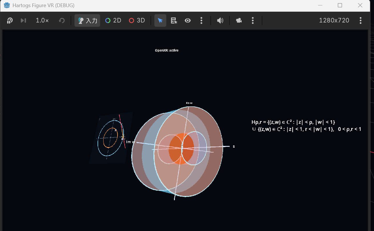
When introducing Hartogs extension, could it help to see where the disk fibres and annular fibres lie? We built this view for learners who have studied one-variable complex analysis and the basics of holomorphic functions of several variables, with the idea of using it alongside a mathematical explanation.
ハルトークス拡張を説明するとき、円板になるファイバーと円環になるファイバーがどこにあるかを、目の前で見られたらどうでしょう。一変数の複素解析と多変数の正則関数の基本を学んだ人への導入を念頭に、講師が説明しながら使える表示を作りました。
We keep the whole \(w\)-plane so that the picture can be related to the usual argument using a contour integral in \(w\). The moving slice shows how the two types of fibre are arranged, rather than reducing each fibre to a radius.
\(w\) 変数の円周積分を使う通常の議論と図を結び付けるため、\(w\) 平面を丸ごと残しています。ファイバーを半径だけに縮めず、円板と円環の配置を、切り方を変えながら眺めます。
How do we draw it?どう描いている?
Write \(\Delta_t=\{\zeta\in\mathbb C:|\zeta|<t\}\) and \(\Delta=\Delta_1\). We use the Hartogs figure
\(\Delta_t=\{\zeta\in\mathbb C:|\zeta|<t\}\)、\(\Delta=\Delta_1\) と書き、次のハルトークス図形を使います。
The parameters \(\rho,r\) are fixed while we observe the figure. We cut the \(z\)-plane with a real line:
\(\rho,r\) は観察中は固定し、\(z\) 平面を次の実直線で切ります。
Here \(a\) translates the line in its normal direction, and \(\theta\) is the angle of the normal. With \(w=u+iv\), the 3D coordinates are \((s,u,v)\). Thus each position along the line retains a whole \(w\)-plane.
\(a\) は法線方向の平行移動量、\(\theta\) は法線の角度です。\(w=u+iv\) と書き、3D表示には \((s,u,v)\) を使います。直線に沿った各位置に、\(w\) 平面がそのまま残ります。
The small \(z\)-plane shows the two circles \(|z|=\rho\), \(|z|=1\) and the current line. In the larger view, translucent boundary surfaces and a few representative fibres make it easier to compare disks and annuli.
小さな \(z\) 平面には \(|z|=\rho\)、\(|z|=1\) の二つの円と、現在の切断直線を表示します。大きな3D図では、半透明の境界面と代表的なファイバーを使って、円板になる部分と円環になる部分を見比べられるようにしています。
Moving the cut, comparing the fibres切り方を動かして、ファイバーを見比べる
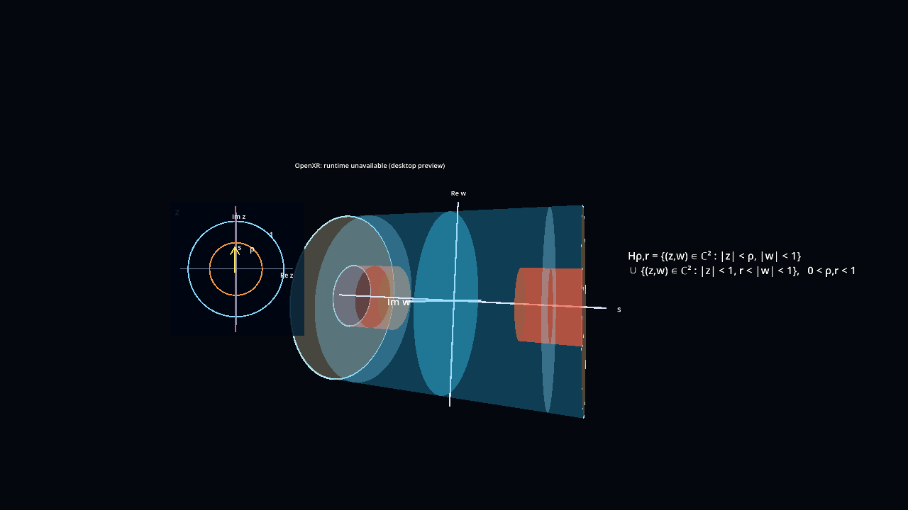
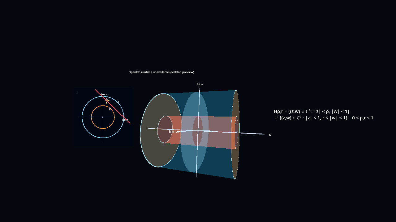
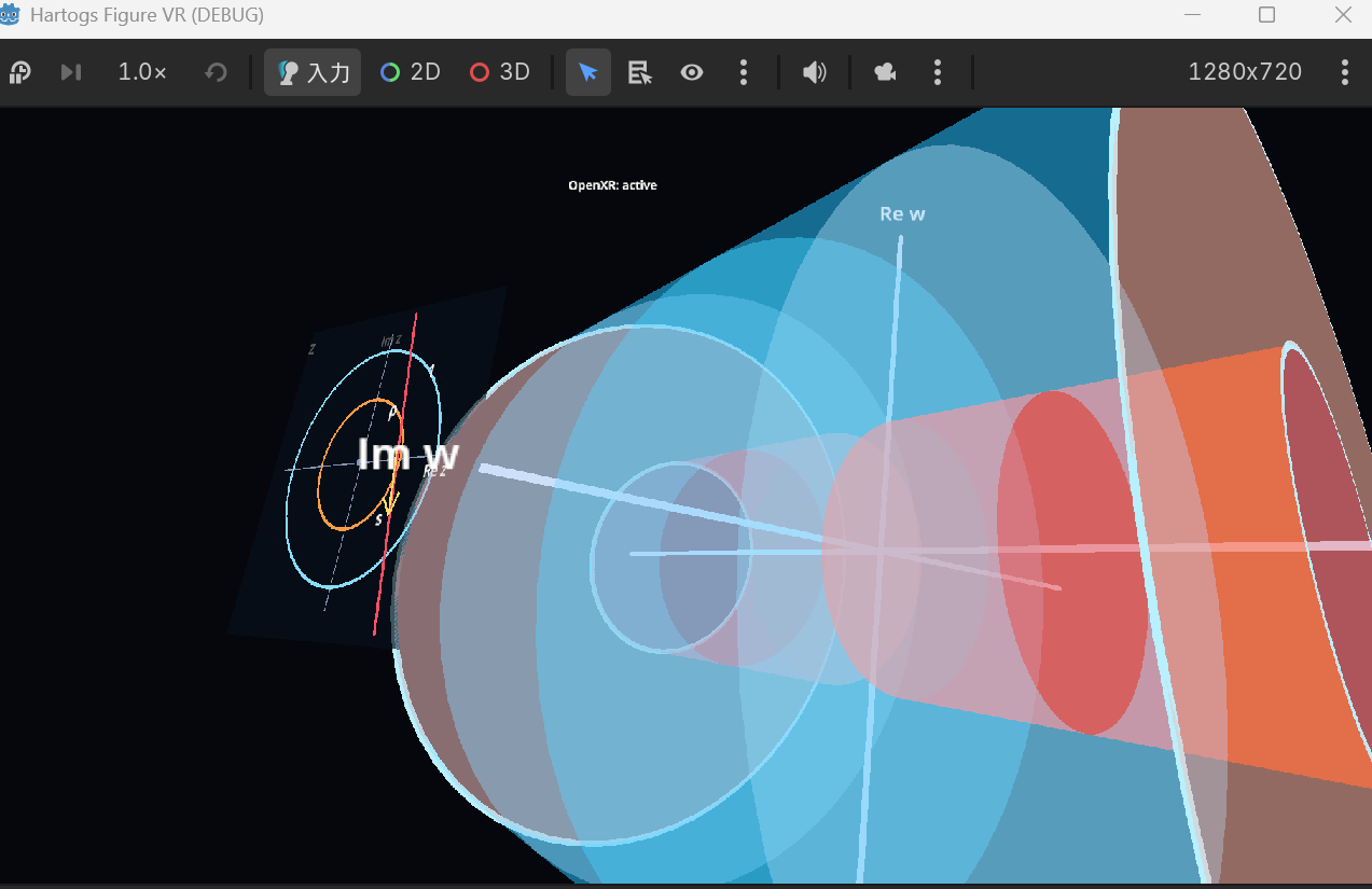
The right stick moves the line: left and right change \(a\), while up and down change \(\theta\). We can compare the small diagram with the corresponding 3D slice as we move it.
右スティックの左右で \(a\) を、上下で \(\theta\) を動かします。小さな図の切断直線と、それに対応する3D断面を見比べながら操作できます。
At a fixed \(s\), the \(w\)-fibre is a disk if \(a^2+s^2<\rho^2\), an annulus if \(\rho^2\leq a^2+s^2<1\), and empty otherwise. When the line stops meeting the inner circle, the disk interval disappears and only annular fibres remain.
\(s\) を固定すると、\(a^2+s^2<\rho^2\) では \(w\) ファイバーは円板、\(\rho^2\leq a^2+s^2<1\) では円環、それ以外では空です。切断直線が内側の円から外れると、円板になる区間がなくなり、円環のファイバーだけが残ります。
We also wanted learners to compare what changes and what stays the same as the line rotates. Rather than display the conclusion automatically, we leave the line and the 3D view side by side for observation and discussion.
直線を回転させたときに何が変わり、何が変わらないかも、二つの図を比べて考えてほしい点です。結論を先回りして表示するのではなく、切断直線と3D図を並べ、観察しながら議論できるようにしました。
How did we build it with Chapio-kun?ちゃぴおくんと、どう作った?
When I explained the mathematical idea to Chapio-kun, my starting reference was Wakabayashi’s 多変数関数論 (Several Complex Variables; in Japanese), volume 21 of 数学のかんどころ. I used it as a reference for the Hartogs-extension argument and explained which arrangement of disks and annuli I wanted to see.
この可視化を相談するとき、私がハルトークス拡張の説明の出発点として参考にしたのは、若林功『多変数関数論』(数学のかんどころ21)です。その議論で見たい円板・円環の配置を、ちゃぴおくんに説明しました。
We asked Chapio-kun to reuse the VR foundation and display the Hartogs figure in its place. Our instructions concerned the mathematics and the interaction: keep the whole \(w\)-plane, move a line in the \(z\)-plane, and show the current cut in a small accompanying diagram.
ちゃぴおくんには、既に作ったVR基本構成を使い、今回はハルトークス図形を表示したいと頼みました。こちらから伝えたのは、\(w\) 平面を丸ごと残すこと、\(z\) 平面の切断直線を動かすこと、現在の切り方を小さな図に示すことでした。
We also discussed the intended lesson, where to put the definition, and why the display should leave room for learners to notice relationships themselves. Chapio-kun turned the discussion into a brief for Codex and helped with the code. Colour, transparency, placement and detailed controls could be proposed and adjusted without us first learning the programming needed to build the scene. We compared the resulting view with the mathematical idea we had described, then discussed further changes.
どんな説明に使いたいか、定義式をどこに置きたいか、学習者の気づきを先回りしない表示にしたいことも相談しました。ちゃぴおくんにCodexへの依頼資料をまとめてもらい、コードの実装も頼みました。色・透明度・配置や細かな操作は、提案してもらいながら調整しています。画面を作るためのプログラミングを先に習得するのではなく、できた表示を当初の数学的な意図と見比べ、次の調整を相談する進め方です。
How would we like to use it?この先、どう使いたい?
We would like to use this view while explaining the contour-integral argument in \(w\), and the step where the extension agrees with the original function on \(|z|<\rho\). The aim is to let the picture and the mathematical argument refer to the same fibres and regions.
今後は、この図を見せながら \(w\) 変数の円周積分を説明し、\(|z|<\rho\) の部分で元の関数との一致を見る議論へつなげたいと考えています。図のどのファイバー、どの部分を使っているのかを、数学の説明と結び付けることが目標です。
For now, the view provides a moving slice and a map of where that slice lies. We want to explore how useful this simple combination is in teaching before adding more features.
現在の表示は、動く断面と、その断面をどこで取っているかを示す図の組合せです。機能を増やす前に、この組合せが説明や観察にどう役立つかを試していきたいと思います。
The initial request and references初回依頼資料と参考文献
These files were prepared with Chapio-kun from our discussion; the TeX version was formatted from an earlier Markdown draft. They are not a verbatim conversation or a single prompt copied from the app. Sections about connecting to the existing project and technical constraints were also prepared with AI assistance. I did not have to know how to write those sections before trying the visualization.
ちゃぴおくんとの対話をもとに整理した初回依頼資料です。先のMarkdown原案をTeXの体裁に整えたもので、逐語録や一度に入力した依頼文そのものではありません。「既存プロジェクトとの接続と作業上の制約」などの技術的な指示も、AIにまとめてもらったものです。私が先にその書き方を知っていなければ始められなかった、ということではありません。
Some technical details and references in the brief have not yet been fully read or checked by me. We are preserving the files as records of the request rather than rewriting them to match this page. Their references may therefore differ from my original reference and the further reading below. See also how to read the implementation briefs.
資料中の技術的な細部や参考文献には、私がまだ読み切れていない・確認できていない部分もあります。依頼の経緯を残すためファイルはそのまま掲載し、出発点にした文献と追加の読書案内は、このページで分けて示します。依頼資料の読み方もご覧ください。
My starting reference出発点にした文献
若林 功『多変数関数論』、数学のかんどころ21、共立出版、2013年。
Wakabayashi, 多変数関数論 (Several Complex Variables; in Japanese), 数学のかんどころ, vol. 21, Kyoritsu Shuppan, 2013.
Further readingさらに背景を読むために
For a detailed account of the Hartogs figure and an approach to extension through the \(\bar\partial\) equation, I also recommend Demailly’s lecture notes. In the version dated 21 June 2012, see Chapter I, (6.3), pp. 45–46, and (3.28), p. 28.
ハルトークス図形による説明や、\(\bar\partial\) 方程式等現代的な方向からのハルトークス型拡張定理については、Demailly氏のレクチャーノートが詳しく、読みやすいと思います。2012年6月21日版では、第I章(6.3)、45–46頁と、(3.28)、28頁等が参考になります。
J.-P. Demailly, Complex Analytic and Differential Geometry, version of 21 June 2012.
Beyond this figure, Ohsawa’s work uses \(L^2\) methods to extend the Kugelsatz-type Hartogs phenomenon to certain domains in Kähler manifolds. See the paper below, as well as the related discussion in his book.
さらに、いわゆるKugelsatz型のハルトークス拡張をKähler多様体上のある種の領域へ広げる方向には、\(L^2\) 理論を用いた大沢氏による一般化があります。以下の論文を挙げますが, 以下の教科書の対応する解説も大変参考になります。
- T. Ohsawa, “Hartogs type extension theorems on some domains in Kähler manifolds”, Annales Polonici Mathematici 106 (2012), 243–254.
- T. Ohsawa, \(L^2\) Approaches in Several Complex Variables: Development of Oka–Cartan Theory by \(L^2\) Estimates for the \(\bar\partial\) Operator, Springer, 2015.
A reference added to the brief by Chapio-kunちゃぴおくんが依頼資料に挙げた文献
Aleksander Simonič, Elementary approach to the Hartogs extension theorem, arXiv:1608.00950.
Simonič’s paper is the reference listed in the AI-prepared brief, whereas Wakabayashi’s book was my starting reference when explaining the mathematics. The brief is left unchanged, rather than replacing its bibliography after the fact.
掲載した依頼資料には、ちゃぴおくんが挙げたSimoničの論文が参考文献として残っています。私が最初の数学的な説明の参考にしたのは、上記の若林の本です。制作過程の記録として、依頼資料の文献は後から入れ替えずに残しています。
The setup guide describes the route to a first VR scene; Notes explains our use of AI.