Levi-flat VR: exploring the holonomy of Levi foliations

From the Levi problem to the foliation of a boundaryLevi問題から、境界の葉層へ

The Levi problem for domains in \(\mathbb C^n\) and unramified Riemann domains over it leads to corresponding questions in general complex manifolds. In complex surfaces, relatively compact Stein or strongly 1-convex domains can have smooth Levi-flat boundaries. We would like to picture how the global analytic properties of such a domain relate to the foliation of its boundary.

複素ユークリッド空間 \(\mathbb C^n\) の領域や、その上の非分岐リーマン領域でのLevi問題を出発点に、一般の複素多様体内の領域へと研究が広がっています。複素曲面内には、滑らかなLevi平坦境界をもつ相対コンパクトなStein領域や強1-凸領域が存在します。そのような領域の大域的な解析的性質と、境界の葉層の振る舞いを結び付けて眺めてみたいと思いました。

A smooth real hypersurface whose Levi form vanishes identically on its complex tangent directions is called a Levi-flat hypersurface. In a complex surface, its complex curves form the Levi foliation. Below, we first introduce the Diederich–Ohsawa disc-bundle example, then the construction of Nemirovski-type hypersurfaces. Our aim was to observe monodromy in the first case and holonomy along compact leaves in the second.

複素接方向でLevi形式が恒等的に0となる滑らかな実超曲面を、Levi平坦超曲面と呼びます。複素曲面内では、複素曲線を葉とするLevi葉層をもちます。以下では、まずDiederich–Ohsawaの円板束の例、次にNemirovski型の構成を取り上げます。前者ではモノドロミー、後者ではコンパクト葉に沿うホロノミーを見る試みです。

Monodromy in the Diederich–Ohsawa exampleDiederich–Ohsawaの例のモノドロミー

To relate a Levi-flat hypersurface in a projective surface to the pseudoconvexity of the domains on its two sides, we wanted to examine the following example studied by Diederich and Ohsawa.

射影曲面の中のLevi平坦超曲面を、その両側の領域の擬凸性と結び付けて眺めるため、Diederich–Ohsawaが扱った次の例を見たいと考えました。

Write \(\mathbb H^+,\mathbb H^-\) for the upper and lower half-planes, and let \(\Sigma=\mathbb H^+/\Gamma\) be a compact Riemann surface of genus at least two, uniformized by \(\Gamma\subset\mathrm{PSL}(2,\mathbb R)\). Using the same action on both factors, set

上半平面・下半平面を \(\mathbb H^+,\mathbb H^-\) とし、種数2以上のコンパクトリーマン面を、一意化するフックス群 \(\Gamma\subset\mathrm{PSL}(2,\mathbb R)\) を用いて \(\Sigma=\mathbb H^+/\Gamma\) と書きます。両因子に同じ作用を用いて、次を作ります。

\begin{gathered} X=(\mathbb H^+\times\mathbb P^1)/\Gamma,\\ M=(\mathbb H^+\times\mathbb{RP}^1)/\Gamma,\\ \gamma\cdot(z,w)=(\gamma z,\gamma w). \end{gathered}

The space \(X\) is a \(\mathbb P^1\)-bundle over \(\Sigma\) and is a projective surface. The compact real-analytic Levi-flat hypersurface \(M\) separates it into two disc bundles:

\(X\) は \(\Sigma\) 上の \(\mathbb P^1\)-束であり、射影曲面です。その中の \(M\) はコンパクトな実解析的Levi平坦超曲面で、補集合は二つの円板束に分かれます。

\begin{gathered}X\setminus M=\Omega^+\sqcup\Omega^-,\\ \Omega^\pm=(\mathbb H^+\times\mathbb H^\pm)/\Gamma.\end{gathered}

Both domains satisfy the pseudoconvexity condition called Takeuchi 1-convexity in \(X\). Diederich and Ohsawa establish this property for the example. [Diederich–Ohsawa]

この両側の領域が、\(X\) 内でTakeuchi 1-凸という擬凸性条件を満たします。 これはDiederich–Ohsawaによって示されています。[Diederich–Ohsawa]

The smooth Levi-flat boundary of a Takeuchi 1-convex domain has no compact leaves. Adachi explains this through leafwise positivity of the normal bundle, using a result of Ohsawa–Sibony. [Adachi]

Takeuchi 1-凸な領域の滑らかなLevi平坦境界には、コンパクト葉は存在しません。足立氏の論文では、Ohsawa–Sibonyの結果を介して、法束の葉方向の正性という観点からこのことが説明されています。[Adachi]

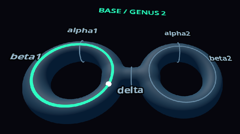
The Levi foliation is induced by the horizontal leaves in \(\mathbb H^+\times\mathbb{RP}^1\). Following a leaf around a loop in \(\Sigma\) gives monodromy on the transverse circle. For a suspension over a compact base, compact leaves correspond to finite orbits of the whole monodromy group. Thus, although individual nontrivial loops in this example have fixed points, there is no finite orbit for the whole group. We wanted to compare how different loops move transverse points, with this connection between pseudoconvexity and the foliation in mind.

Levi葉層は、\(\mathbb H^+\times\mathbb{RP}^1\) の水平な葉から誘導されます。底空間 \(\Sigma\) のループに沿って葉をたどると、横断円周上にモノドロミーが現れます。コンパクトな底空間上のsuspensionでは、コンパクト葉があることは、モノドロミー群全体の有限軌道があることに対応します。この例では個々の非自明なループに固定点があっても、作用全体には有限軌道がありません。このような擬凸性と葉層の関係を念頭に、異なるループのモノドロミーが横断方向の点をどう動かすか、実際に見比べたいと考えました。

The representation we intended to visualize, and the one we used可視化したかった表現と、実際に用いた表現

My intended starting point was a discrete faithful representation of the genus-two surface group. Taking the quotient of the upper half-plane by its image would specify the base Riemann surface, and using the same action on the fibre would give the diagonal-action example above. Faithfulness alone is not the full requirement: discreteness is needed as well.

本来使いたかったのは、種数2曲面群の離散忠実表現でした。その像で上半平面を割って底のリーマン面を定め、同じ作用をファイバーにも用いれば、先に説明した対角作用の例になります。ここでは、忠実性だけでなく離散性も必要です。

\rho_{\mathrm F}:\pi_1(\Sigma_2)\longrightarrow\mathrm{PSL}(2,\mathbb R)

During my master's studies, a friend had told me that such a representation could be written quite explicitly. Remembering this, I asked Chapio-kun to find references, choose a concrete representation, and turn the plan into a TeX implementation brief. In retrospect, I may have shifted towards asking for a representation that was easy to draw without keeping the requirement of discreteness and faithfulness sufficiently explicit.

修士の頃、友人から、そのような表現を具体的に分かりやすく書けると教わった記憶がありました。そこで、文献を探して具体的な表現を選び、それを固定した実装依頼資料をTeXでまとめてもらうつもりで、ちゃぴおくんに相談しました。振り返ると、私自身、途中から描画しやすい表現という希望を中心に話し、離散忠実性の条件を十分に明示し続けていなかったのかもしれません。

The generated brief instead proposed the following matrices to simplify calculation and rendering. It explicitly distinguished this choice from a uniformizing representation and deferred that representation to future work. I proceeded to implementation without fully recognizing the change of target, and noticed the mismatch only after the VR graphics were complete, when I examined what I had seen more closely.

生成された依頼資料では、計算・描画の簡単さを優先して次の行列が提案されていました。一意化表現とは異なることも記され、本来の一意化表現を使う模型は将来の作業へ回されていました。私は対象が変わっていることを十分に認識しないまま実装を進め、3D VRグラフィックが完成して観察した後、見えたものの解釈を詳しく検討する段階で、この齟齬に気付きました。

Cropped original screenshot of the genus-two base navigator, with labels alpha1, beta1, alpha2, beta2 and delta. — A topological guide to the loops \(\alpha_1,\beta_1,\alpha_2,\beta_2,\delta\) on the genus-two base, used to select the monodromy shown in the suspension view.種数2の底空間のループ \(\alpha_1,\beta_1,\alpha_2,\beta_2,\delta\) を選ぶ位相的な案内図。選んだループに沿うモノドロミーを、suspensionの表示で見比べます。

\begin{gathered}\pi_1(\Sigma_2)=\langle\alpha_1,\beta_1,\alpha_2,\beta_2\mid\\{}[\alpha_1,\beta_1][\alpha_2,\beta_2]=1\rangle,\\\rho:\pi_1(\Sigma_2)\longrightarrow\mathrm{PSL}(2,\mathbb R).\end{gathered}

A=\begin{pmatrix}2&1\\1&1\end{pmatrix},\qquad B=\begin{pmatrix}2&-1\\-1&1\end{pmatrix}.

\begin{aligned}\rho(\alpha_1)&=A,&\rho(\beta_1)&=B,\\\rho(\alpha_2)&=B,&\rho(\beta_2)&=A.\end{aligned}

With the convention \([A,B]=ABA^{-1}B^{-1}\), the surface-group relation is satisfied because \([A,B][B,A]=I\). However, there are also the relations

交換子を \([A,B]=ABA^{-1}B^{-1}\) とすれば、\([A,B][B,A]=I\) により曲面群の関係式は満たします。しかし同時に、次の関係もあります。

\rho(\alpha_1\beta_2^{-1})=1,\qquad \rho(\beta_1\alpha_2^{-1})=1.

Both words are nontrivial in the surface group: their images are nonzero even in its abelianization \(H_1(\Sigma_2;\mathbb Z)\simeq\mathbb Z^4\). Thus \(\rho\) is not faithful. The resulting suspension is not the Diederich–Ohsawa diagonal-action example I intended to reproduce. Satisfying the surface-group relation did not suffice to select a uniformizing representation. The Takeuchi 1-convexity conclusion above cannot simply be transferred to this representation.

この二つの語は、曲面群のアーベル化 \(H_1(\Sigma_2;\mathbb Z)\simeq\mathbb Z^4\) でも非零なので、曲面群では非自明です。したがって \(\rho\) は忠実ではありません。でき上がったsuspensionは、再現したかったDiederich–Ohsawaの対角作用の例とは異なります。 曲面群の関係式を満たすことだけでは、一意化表現を選べたことにはなりませんでした。上で述べたTakeuchi 1-凸性の結論を、この表現へそのまま移すこともできません。

The matrices do define a suspension: the surface group acts by covering transformations on the universal cover of the base and by \(\rho\) on the fibre. We retain its images and the original brief as a record of the attempt, including this mismatch in the choice of target.

この行列でも、底の普遍被覆には被覆変換として、ファイバーには \(\rho\) で作用させることで、suspension自体は作れます。ここでは当初の画像と依頼資料を変えずに残し、目標とした対象の選択に齟齬があったことも含めて報告します。

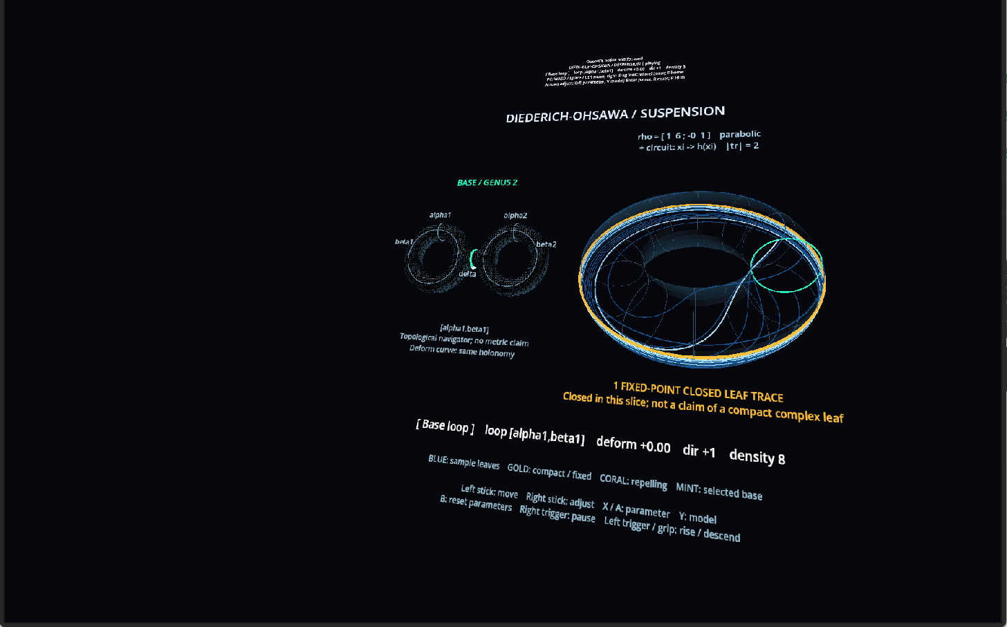
For the representation actually used, \(A,B\) are hyperbolic with disjoint fixed-point sets. The whole action therefore has no finite orbit: any point in one would be periodic, hence fixed, under both matrices. For \(\delta=[\alpha_1,\beta_1]\), we have

実際に用いた表現でも、\(A,B\) は双曲型で、固定点集合は交わりません。作用全体に有限軌道もありません。有限軌道の各点は両行列の周期点、したがって共通固定点になるはずだからです。\(\delta=[\alpha_1,\beta_1]\) については、

[A,B]=-\begin{pmatrix}1&6\\0&1\end{pmatrix}.

This represents the parabolic map \(t\mapsto t+6\) on \(\widehat{\mathbb R}\), with the single fixed point \(\infty\). A Cayley transform transfers these real projective actions to the circle.

これは \(\widehat{\mathbb R}\) 上の放物型の写像 \(t\mapsto t+6\) を表し、固定点は \(\infty\) 一つです。これらの実射影直線上の作用を、Cayley変換で円周上の作用へ移して表示します。

In a uniformizing group for a compact surface, every nontrivial element is hyperbolic; the parabolic behaviour shown for \(\delta\) here is another indication of the mismatch.

コンパクト曲面を一意化する群では、非自明な元はすべて双曲型です。ここで \(\delta\) に現れる放物型の振る舞いも、意図した例との違いです。

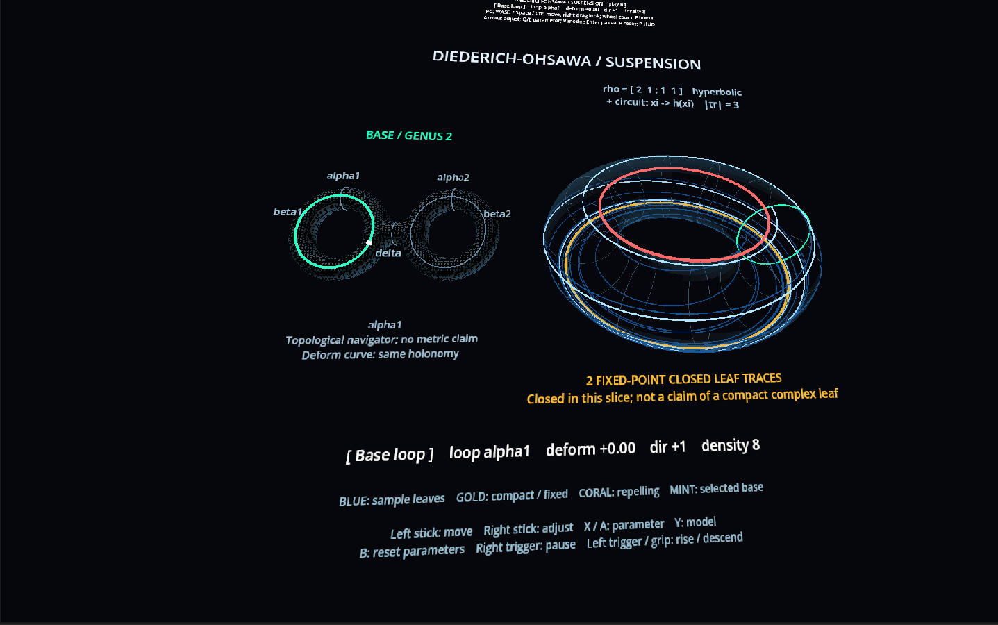
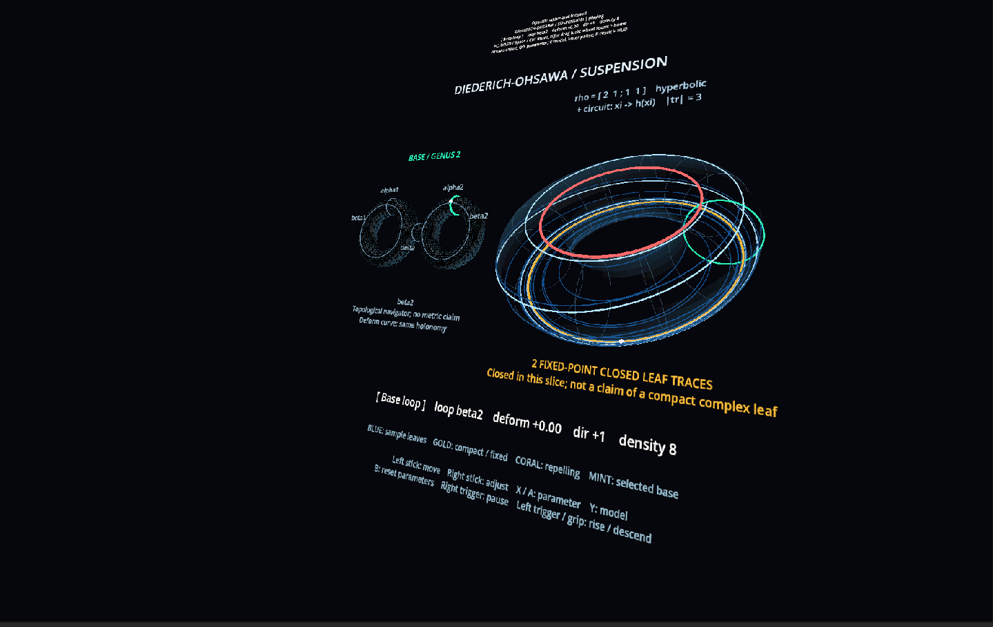
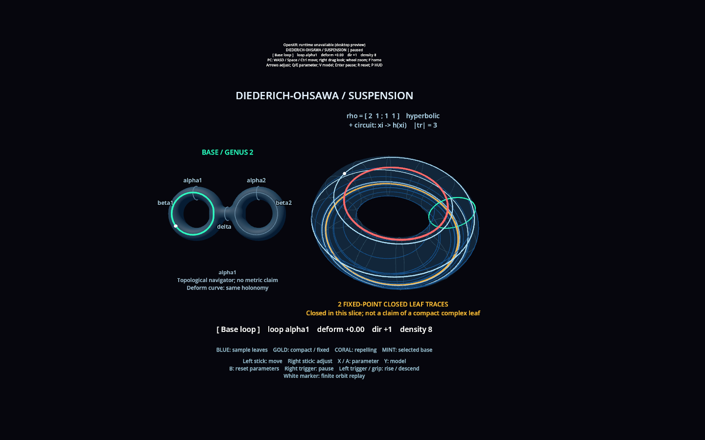
K(t)=\frac{t-i}{t+i},\qquad h_\gamma=K\circ\rho(\gamma)\circ K^{-1}.

The right-hand view is the restriction to the selected loop, with the identification

右側の画面は、選んだループ上への制限で、次の貼り合わせを表示しています。

([0,1]\times S^1)\big/\big((1,\xi)\sim(0,h_\gamma(\xi))\big).

The gold and coral closed curves trace fixed points of this monodromy; the blue curves trace other points. They are intersections of leaves with the surface over the loop. Changing the loop lets us compare the actions on the transverse circle.

金色・珊瑚色の閉曲線はそのモノドロミーの固定点の軌跡、青い曲線は他の点の軌跡です。いずれも、ループ上の曲面で切り出した葉の軌跡を表します。ループを切り替え、横断円周への作用を見比べます。

Holonomy along compact leaves of Nemirovski-type Levi-flat hypersurfacesNemirovski型Levi平坦超曲面のコンパクト葉に沿うホロノミー

Nemirovski’s 1999 construction gives compact complex surfaces separated by a smooth Levi-flat hypersurface into two Stein domains. The boundary nevertheless contains compact leaves. It therefore provides a useful contrast: Steinness of the complementary domains alone does not rule out compact leaves in the boundary. [Nemirovski]

Nemirovskiが1999年に与えた構成は、コンパクト複素曲面を滑らかなLevi平坦超曲面で二つのStein領域へ分ける例です。その境界にはコンパクト葉が含まれます。補集合の領域がSteinであることだけでは境界のコンパクト葉を排除できない、という点でも、先の例との対比が興味深いところです。［Nemirovski］

From a meromorphic section to a Levi-flat hypersurface有理型切断からLevi平坦超曲面を作る

We use the line-bundle construction on p. 379 of Ohsawa’s 2006 supplement, following its notation. Let \(C\) be a compact Riemann surface, \(L\to C\) a holomorphic line bundle, and \(s\) a nonzero meromorphic section with only simple zeros and simple poles. Write \(C'\) for the complement of those zeros and poles, \(L'\) for the complement of the zero section in \(L\), and \(\mathbb R'=\mathbb R\setminus\{0\}\). We assume \(C'\ne C\). [Ohsawa]

以下では、大沢氏の2006年の補遺の379頁にある、直線束からの構成とその記号に沿います。\(C\) をコンパクトリーマン面、\(L\to C\) を正則直線束とし、単純零点・単純極だけをもつ非零有理型切断 \(s\) を取ります。零点・極を除いた底空間を \(C'\)、\(L\) から零切断を除いたものを \(L'\)、\(\mathbb R\setminus\{0\}\) を \(\mathbb R'\) と書き、\(C'\ne C\) とします。［Ohsawa］

Choose a positive real multiplier \(a>1\) (labelled \(r\) on screen), let \(\mathbb Z\) act fibrewise by multiplication by \(a^m\), and set

実数 \(a>1\)（画面のパラメータ \(r\)）を選び、各ファイバー上で \(a^m\) を掛ける \(\mathbb Z\) 作用により、次を作ります。

\begin{gathered}X=L'/a^{\mathbb Z},\qquad \pi:X\longrightarrow C,\\M=\overline{\{[\lambda s(p)]\mid p\in C',\ \lambda\in\mathbb R'\}}\ \subset X.\end{gathered}

Over \(C'\), the section \(s\) trivializes \(L\). In this trivialization the fibre coordinate is \(q=w/s(z)\), and the construction gives

\(C'\) 上では \(s\) により \(L\) を自明化できます。そのファイバー座標を \(q=w/s(z)\) とすると、構成式から次が分かります。

\begin{aligned}M\cap\pi^{-1}(C')&\simeq C'\times(\mathbb R'/a^{\mathbb Z})\\&\simeq C'\times(S^1\sqcup S^1).\end{aligned}

Thus the hypersurface meets each elliptic fibre in two circles, corresponding to the positive and negative real values of \(q\). The leaves are horizontal in this trivialization: they keep \([q]=[\lambda]\) fixed and are the graphs \(z\mapsto[\lambda s(z)]\). Each such leaf is biholomorphic to \(C'\).

したがって、各楕円ファイバーと超曲面との交わりは、\(q\) の正・負に対応する二つの円周です。Levi葉層の葉は、この自明化では \([q]=[\lambda]\) を一定に保つ水平な曲線で、元の座標では \(z\mapsto[\lambda s(z)]\) というグラフになります。各葉は \(C'\) と双正則です。

The essential step is that taking the closure extends this hypersurface smoothly over the zeros and poles. The entire elliptic fibre over each of them becomes a compact leaf. The other, horizontal leaves accumulate on these compact leaves as they approach the punctures in the base. This is the behaviour we wanted to visualize near a zero and a pole.

重要なのは、閉包を取ることで、この超曲面が零点・極の上にも滑らかに延びることです。 そこでは楕円ファイバー全体がコンパクト葉になります。それまで底空間に対して水平に走っていた非コンパクト葉は、零点・極へ近づくと、これらのコンパクト葉へ巻き付きながら集積します。今回、零点・極の近くで見たいと思ったのは、この振る舞いです。

Extension over a zero or pole, and its holonomy零点・極への延長とホロノミー

Near a simple zero or pole, choose a base coordinate \(z\) and a local frame of \(L\) in which \(s(z)=z\) or \(s(z)=1/z\), respectively. Before taking the quotient, the local equations of the closure are

単純零点・単純極の近くで、底空間の局所座標 \(z\) と \(L\) の局所枠を選ぶと、\(s(z)=z\)、または \(s(z)=1/z\) と書けます。商を取る前の閉包の局所方程式は、それぞれ次の形になります。

\begin{aligned}\widetilde M_0&=\{(z,w):\operatorname{Im}(z/w)=0,\ w\ne0\},\\\widetilde M_\infty&=\{(z,w):\operatorname{Im}(zw)=0,\ w\ne0\},\\ (z,w)&\sim(z,aw).\end{aligned}

Since \(w\ne0\), the derivative with respect to \(z\) of the holomorphic function \(z/w\) or \(zw\) is nonzero even at \(z=0\). These equations therefore define smooth Levi-flat hypersurfaces there. After the quotient, the whole fibre over \(z=0\) is the compact leaf

\(w\ne0\) なので、正則函数 \(z/w\)、\(zw\) の \(z\) 方向の微分は \(z=0\) でも0にならず、ここでも滑らかなLevi平坦超曲面を定めます。商を取ると、\(z=0\) のファイバー全体が、次のコンパクト葉になります。

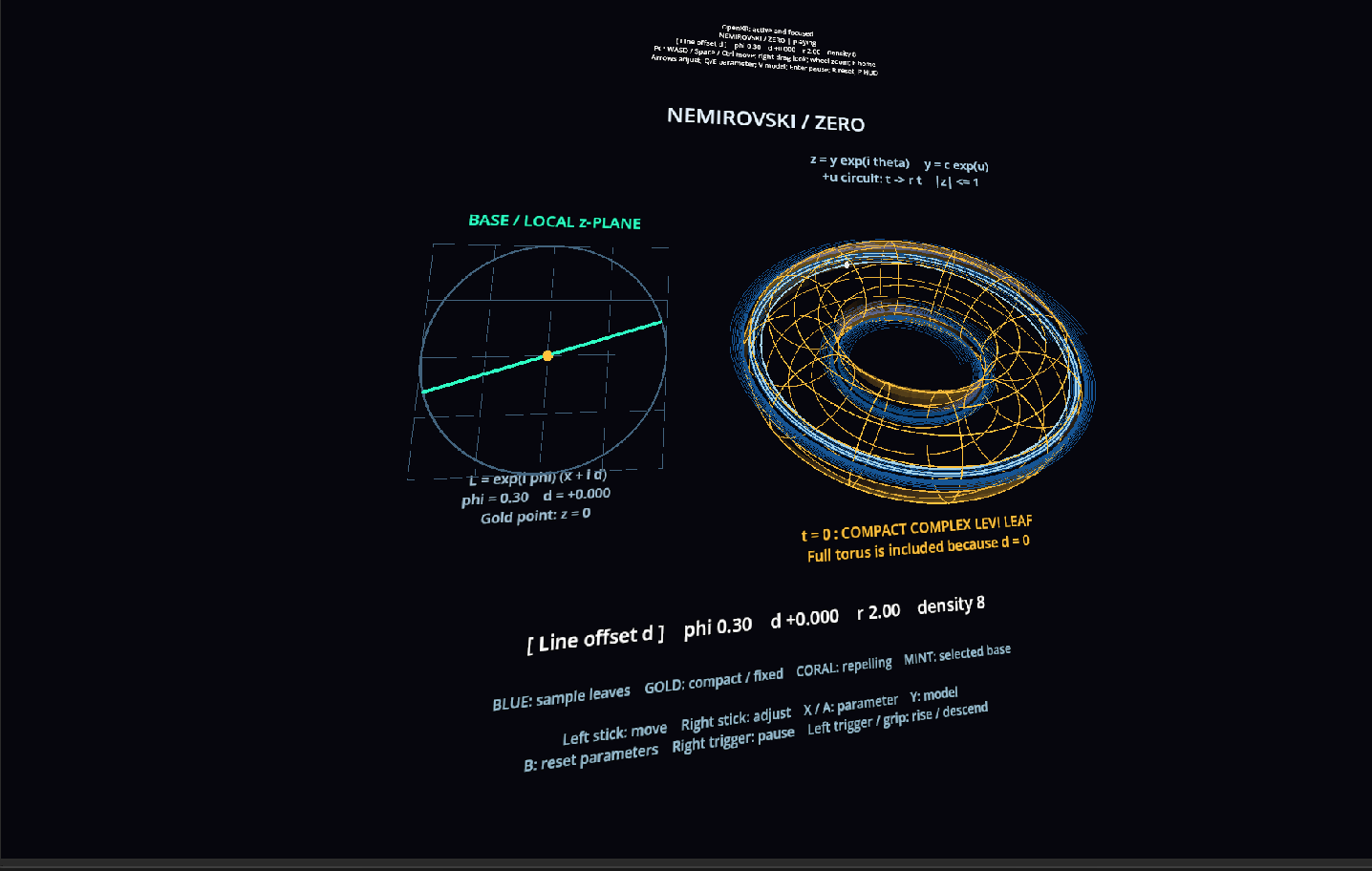
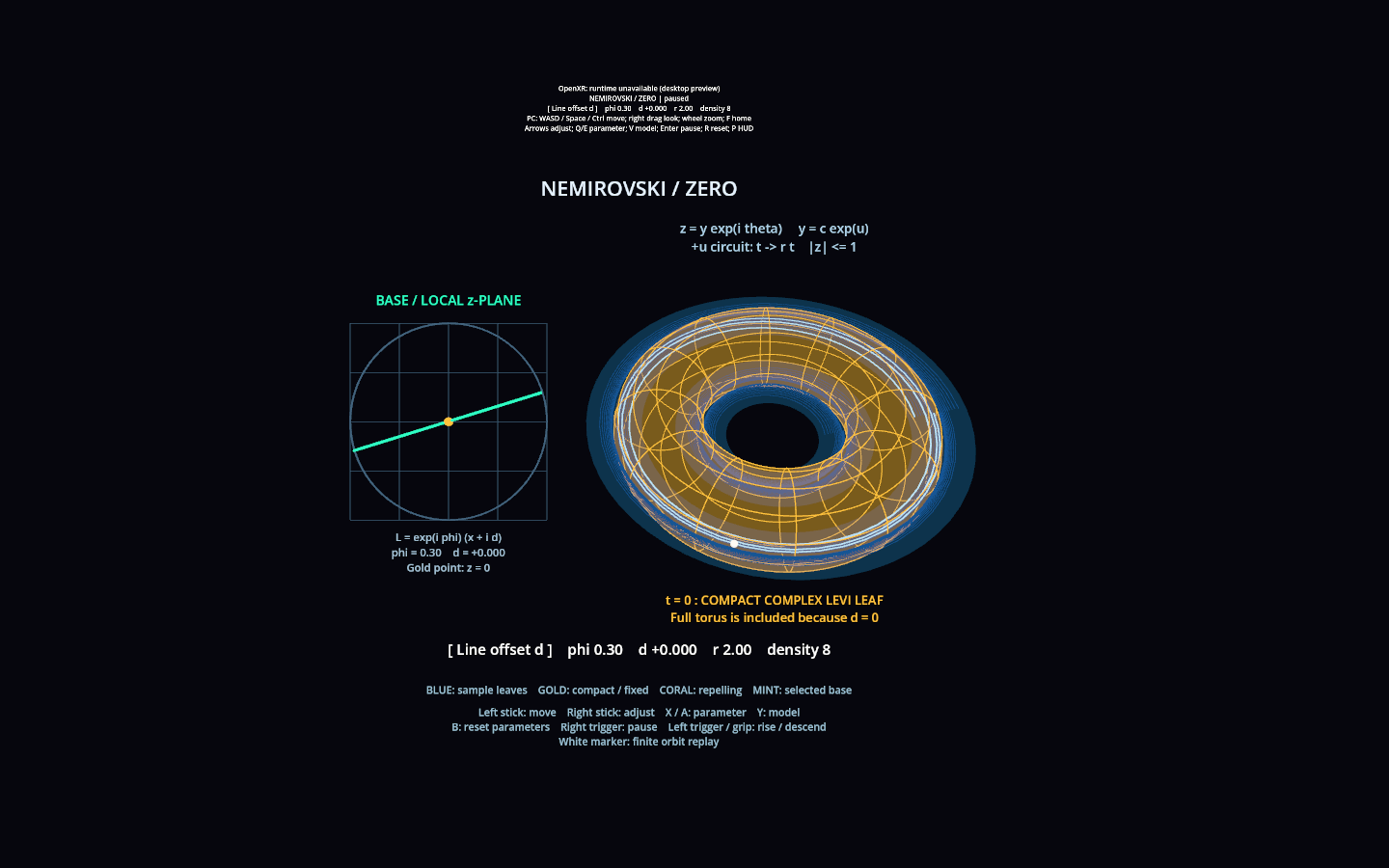
E_a=\mathbb C^\times/a^{\mathbb Z}\simeq\mathbb C/\bigl((\log a)\mathbb Z+2\pi i\mathbb Z\bigr).

On a lift, the leaves are given by constant real \(t=z/w\) in the zero model and constant real \(t=zw\) in the pole model. In both cases \(t=0\) gives \(E_a\). Writing \(w=e^{u+i\theta}\), and taking the loop on the compact leaf with increasing \(u\) as positive, the holonomy germs are

持ち上げた座標では、零点側は \(t=z/w\in\mathbb R\)、極側は \(t=zw\in\mathbb R\) を一定に保つ曲線が葉です。いずれも \(t=0\) が \(E_a\) に対応します。\(w=e^{u+i\theta}\) と書き、コンパクト葉の上で \(u\) が増える向きの周回を正方向に取ると、ホロノミーの芽は

h_0(t)=at,\qquad h_\infty(t)=t/a.

The \(\theta\)-circle has trivial holonomy. Reversing the \(u\)-circle gives the inverse map; in the contracting direction a transverse point follows \(t,t/a,t/a^2,\ldots\). These are loops within the compact leaf. Over \(C'\), by contrast, the product trivialization above has trivial base monodromy.

となります。\(\theta\) を一周させるループのホロノミーは恒等写像です。\(u\) の周回を逆向きにすれば逆写像になり、収縮する向きでは横断方向の点が \(t,t/a,t/a^2,\ldots\) と近づきます。ここで回っているのはコンパクト葉の中のループです。一方、\(C'\) 上では先の積自明化があり、底空間のループに沿うモノドロミーは自明です。

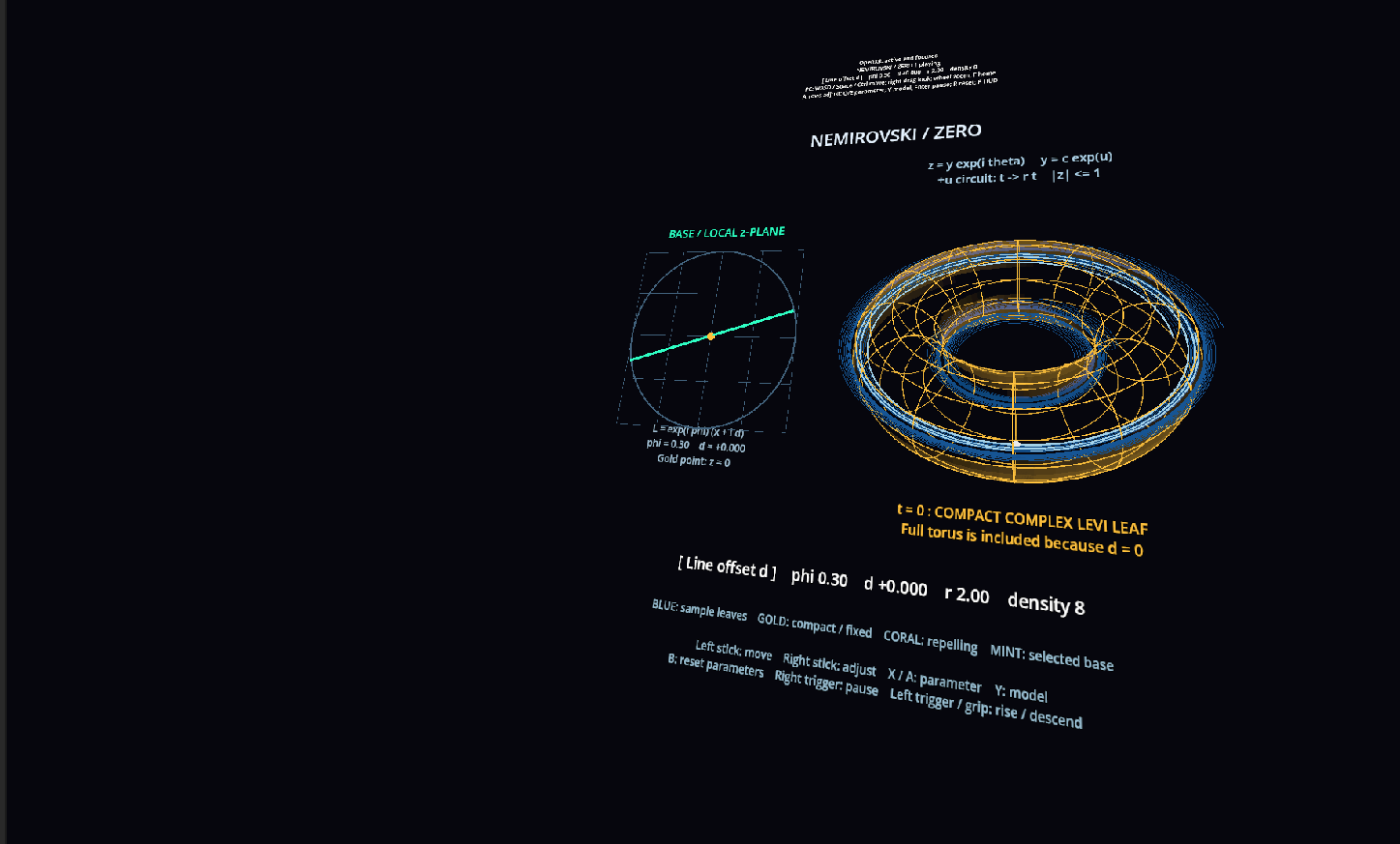
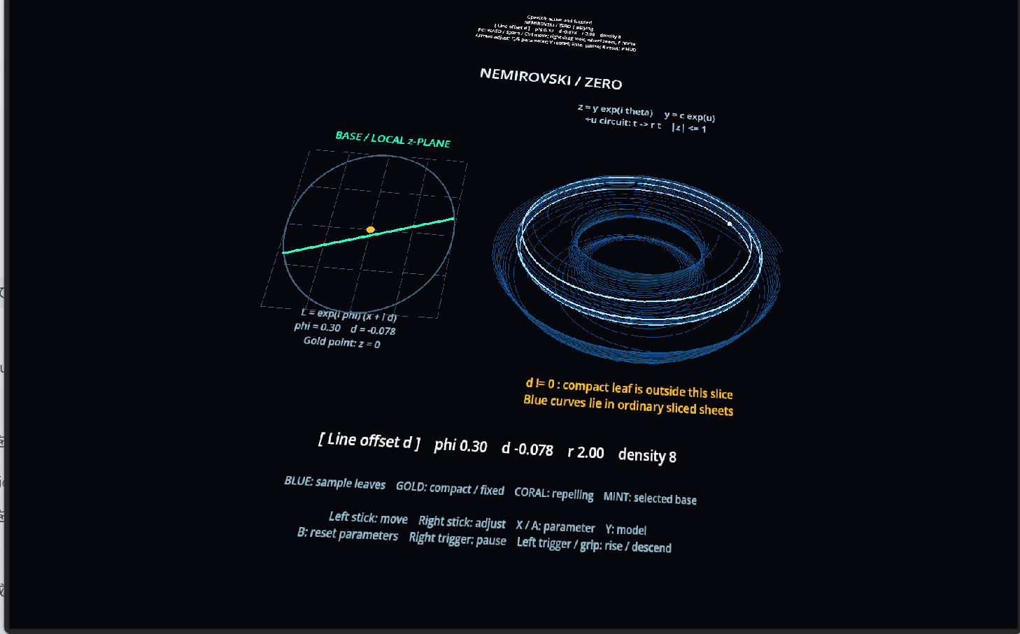
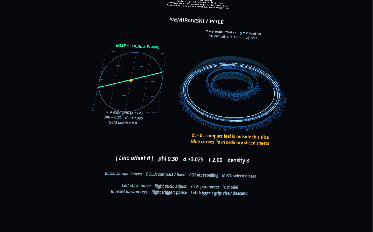
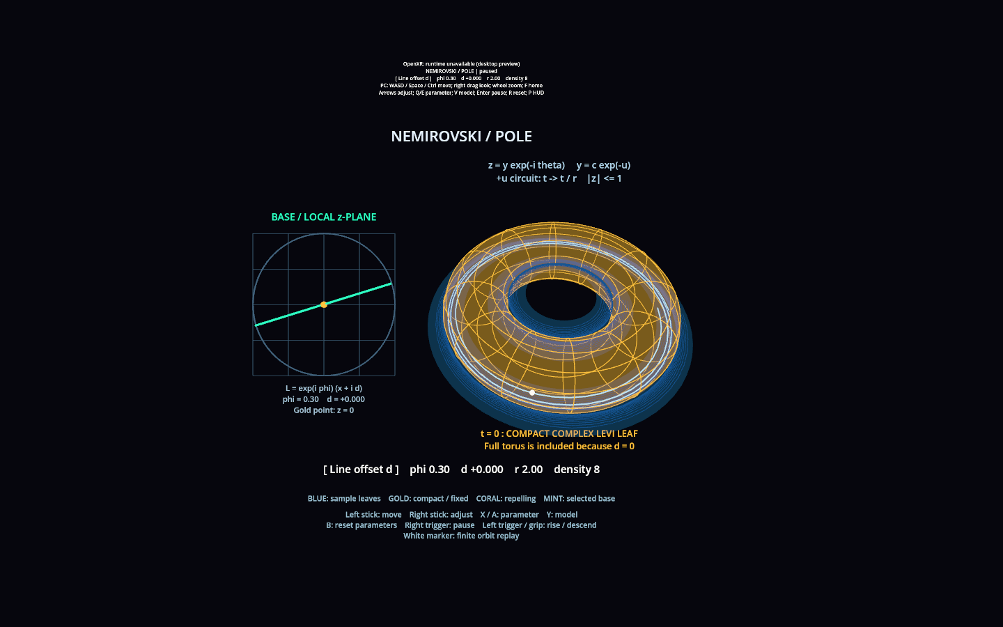
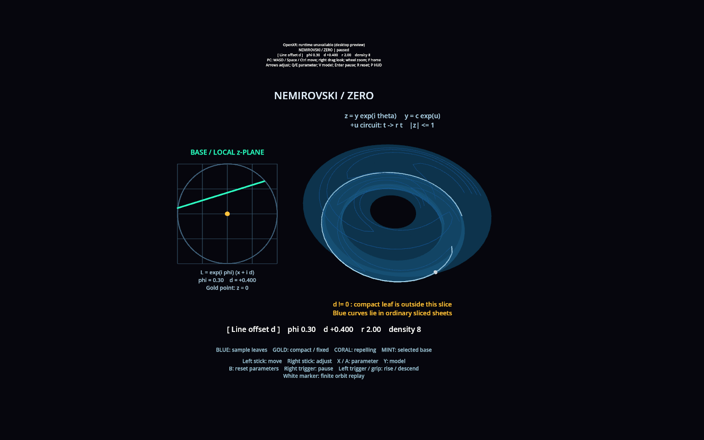
The torus display uses the two periods \(u\bmod\log a\) and \(\theta\bmod2\pi\), coming from the covering transformation \(w\mapsto aw\) and the argument of \(w\), and places the transverse direction around them. We then select a real line in the local base: at \(d=0\) it passes through the zero or pole and includes the whole gold compact leaf; offsetting it cuts out blue traces of other leaves instead.

トーラス表示では、被覆変換 \(w\mapsto aw\) と \(w\) の偏角に由来する二つの周期 \(u\bmod\log a\)、\(\theta\bmod2\pi\) をトーラスの二方向へ対応させ、横断方向をその周囲へ配置しています。さらに底空間の局所座標を実直線で切り、原点を通る断面（\(d=0\)）には金色のコンパクト葉全体を含め、直線をずらした断面では他の葉の青い軌跡を見比べます。

Nemirovski-type zero model: a gold compact leaf and blue traces of nearby leaves at d = 0. — The zero model of a Nemirovski-type Levi-flat hypersurface, at d = 0. The gold torus is the compact leaf over the zero; the blue curves are traces of other leaves in the selected slice.Nemirovski型Levi平坦超曲面の零点模型、d = 0。金色のトーラスは零点上のコンパクト葉、青い曲線は選んだ断面に現れる他の葉の軌跡です。

Comparing slices and loops断面とループを見比べる

Compare a model, a slice and a base loop with the formulas above. The images open at full size; changes of viewpoint and slice position are identified in the captions.

模型・断面・底空間のループを切り替え、上の式と見比べます。画像は押すと大きく開けます。視点や断面の位置が異なるものは、キャプションで区別しています。

Suspension: traces over selected loopsSuspension：選んだループ上の軌跡

Suspension over \(\alpha_1\). Its monodromy is represented by \(A\), with two fixed-point traces in gold and coral.\(\alpha_1\) 上のsuspension。モノドロミーは \(A\) に対応し、二つの固定点の軌跡を金色と珊瑚色で表します。

The \(\beta_2\) view from another position. Its monodromy is also \(A\); these two images do not compare different transformations.別の位置から見た \(\beta_2\) の画面。こちらもモノドロミーは \(A\) なので、この二枚は異なる作用どうしの比較ではありません。

The commutator loop \(\delta\). Its parabolic monodromy has one fixed point, shown by one gold closed trace.交換子のループ \(\delta\)。放物型のモノドロミーには固定点が一つあり、金色の閉じた軌跡が一本現れます。

Nemirovski type: moving the sliceNemirovski型：断面をずらす

The zero model at d = 0. The selected line in the base passes through the origin, so the compact leaf is included.零点模型、d = 0。底空間の切断直線が原点を通り、コンパクト葉が断面に含まれます。

The zero model at d = −0.078. The compact leaf lies outside the selected slice; blue traces remain.零点模型、d = −0.078。コンパクト葉が断面の外に出て、青い軌跡が表示されています。

The pole model at d = +0.025. This is an offset slice, not a zero/pole comparison at matching parameters.極模型、d = +0.025。ずらした断面の画面であり、上の零点模型と条件を揃えた比較ではありません。

Additional desktop views比較のためのPC描画

The following five images were saved separately as desktop rendering previews. In particular, the zero and pole models at d = 0 can be viewed more nearly from the front.

次の五枚は、別途保存したPC描画です。特に d = 0 の零点・極模型を、正面に近い向きから見比べられます。

Desktop preview: zero model, d = 0.PC描画：零点模型、d = 0。

Desktop preview: pole model, d = 0.PC描画：極模型、d = 0。

Desktop preview: zero model, d = 0.4.PC描画：零点模型、d = 0.4。

Desktop preview: hyperbolic monodromy over \(\alpha_1\), with two fixed-point traces.PC描画：\(\alpha_1\) の双曲型モノドロミーと、二つの固定点の軌跡。

Desktop preview: parabolic monodromy over \(\delta\), with one fixed-point trace.PC描画：\(\delta\) の放物型モノドロミーと、一つの固定点の軌跡。

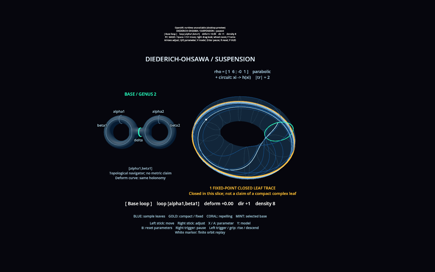
A moving white marker helps us follow sampled traces in the application. Its replay is a display aid, not a claim that the mathematical orbit is periodic. This page presents still images rather than running the VR application in the browser.

アプリの白い点は、サンプルの軌跡をたどるための補助表示です。再生の繰り返しを、数学的な軌道の周期性とは区別します。このページでは静止画を紹介し、ブラウザー内でVRアプリを動かすものではありません。

What I could read from the views見比べて、何が読み取れたか

I returned to the VR views after discussing the mathematics, comparing the two models again.

数学の説明とVRを行き来しながら、改めて二つの表示を見比べました。

When I viewed the VR graphics believing them to depict the Diederich–Ohsawa example, the different monodromies seemed to have no common fixed point, and I felt that transverse points would be “stirred around”. This seemed consistent with what I knew of the example, and I was close to being satisfied with that interpretation.

Diederich–Ohsawaの例を描いたつもりでVRを眺めたとき、異なるループのモノドロミーを見比べると、作用全体に共通する固定点はなさそうで、「横断方向の点がよくかき混ぜられていそうだ」と感じました。知っている例の性質と合うように思え、一度は納得しかけていました。

Checking the matrices more closely afterwards revealed the mismatch described above. The intended example had not been reproduced. The impression of points being stirred around did not distinguish the two representations, and I had not observed mixing or any other more specific dynamical property.

ところが、その後で行列を詳しく確かめると、先に述べた齟齬が分かりました。意図した例は再現できていなかったのです。「よくかき混ぜられそう」という印象だけでは、この違いを見分けられませんでした。また、混合性などの具体的な力学系的性質を観察できたわけでもありません。

I found the rendering and interaction themselves very good, and would like to try again with a discrete faithful uniformizing representation. At the same time, correcting the representation alone may still leave me with little more than the impression that the monodromy looks complicated. I would also like to explore other 3D VR views that might help me grasp distinctive features of the intended example, such as Takeuchi 1-convexity, more intuitively.

表示や操作の仕組み自体はとてもよくできていたと感じており、次は離散忠実な一意化表現に直して、改めて観察したいと思います。一方、表現を直すだけでは、「たしかにモノドロミーが複雑そうだ」という感想以上の理解にはつながらないかもしれない、とも感じました。この例については、Takeuchi 1-凸性などの特徴的な性質を、もっと直観的につかめるような別の3D VR表示の方法も検討してみたいです。

I regard this mismatch as a valuable experience in working with AI. A working implementation and a visualization of the intended mathematical object need to be checked separately. Alongside the code, we need to examine how the assumptions in our request become concrete formulas and parameters. Looking back at those assumptions is an important part of using what we see in VR.

この齟齬も、AIとともに数学的対象を具体化する過程で得られた、よい経験だと捉えています。実装が動いたことと、意図した数学的対象を描けたことは、分けて確かめる必要がありました。AIに具体化を任せるときは、コードだけでなく、こちらの仮定がどの式やパラメータへ置き換えられたかも人間が点検し、見えたものを当初の定義や仮定に立ち返って確かめながら観察したいと思います。

In the Nemirovski-type Levi-flat hypersurface model, I could clearly see the traces of leaves winding around the gold torus representing a compact leaf.

Nemirovski型Levi平坦超曲面では、葉を切り出した軌跡が、コンパクト葉である金色のトーラスの周りへ巻き付いていく様子を、分かりやすく見ることができました。

I also compared the zero and pole models. My first impression was that they did not look very different. Returning to the formulas afterwards, I realized that the two local models are related by the biholomorphic map \((z,w)\mapsto(z,w^{-1})\). Their similar appearance was therefore not surprising—but in this case it was the visual comparison that prompted me to notice the equivalence.

零点側と極側も見比べてみましたが、第一印象は「あまり変わらない」でした。その後で式に戻ると、二つの局所模型は \((z,w)\mapsto(z,w^{-1})\) という双正則変換で移り合います。似た見え方で不思議はなかったわけですが、今回は見比べてから、そのことに気付きました。

This map descends to the quotient and reverses the chosen \(u\)-circle, exchanging the two holonomy formulas.

この写像は商にも降り、選んだ \(u\) の周回方向を逆にするため、二つのホロノミーの式を入れ替えます。

Making it with Chapio-kunちゃぴおくんと、どう作った？

We discussed the two mathematical models and the views we wanted with Chapio-kun, then gave Codex the implementation brief, asking it to reuse the common VR foundation. The detailed placement of the geometry and the controls was worked out during implementation.

二つの数学的な模型と見たい表示をちゃぴおくんと相談し、実装依頼資料をCodexへ渡して、汎用VR基本構成も活用してほしいと頼みました。形状の配置や操作の具体化は、実装の中で進めています。

After the display worked, we compared different slices and loops, returning to the formulas as questions arose. The zero/pole comparison above is one example of that back-and-forth: the visual impression came first, and the local equivalence became clear on returning to the mathematics.

表示できた後も、断面やループを変えて眺め、気になった点を式へ戻って考えました。上の零点・極の比較は、その往復の一例です。先に見た印象があり、数学へ戻ることで局所模型の対応がはっきりしました。

Implementation brief and references実装依頼資料と参考文献

The initial implementation brief is available as PDF and TeX, unchanged. It records the choices that led to the implementation, including the mismatch with the intended representation identified above. We have not rewritten the brief after the fact. For the current interpretation and observations, use this page; see also how to read the implementation briefs.

初回の実装依頼資料を、当時のPDF・TeXのまま掲載しています。先に述べた意図した表現との齟齬も残る制作記録として、後から書き換えていません。現在の解釈や観察については、このページの説明をご覧ください。依頼資料の読み方も参照できます。

Read the brief (PDF, Japanese)実装依頼資料を読む（PDF・日本語）TeX source of the brief依頼資料のTeXファイル

References参考文献

K. Diederich and T. Ohsawa, On the Displacement Rigidity of Levi Flat Hypersurfaces—The Case of Boundaries of Disc Bundles over Compact Riemann Surfaces, Publications of the Research Institute for Mathematical Sciences 43 (2007), 171–180.

For Takeuchi 1-convexity of the diagonal-action example described above, see the proposition on p. 172, deduced from Proposition 1.6. Remark 1.7 on p. 175 explains how to treat the exterior as a disc bundle as well.

本文で挙げた対角作用の例のTakeuchi 1-凸性については、Proposition 1.6から導かれる172頁のPropositionを参照してください。175頁のRemark 1.7では、外側も円板束として扱えることが説明されています。
S. Yu. Nemirovski, Stein domains with Levi-plane boundaries on compact complex surfaces, Mathematical Notes 66 (1999), 522–525.
The introduction and §1 construct a smooth Levi-flat hypersurface separating a compact complex surface into two Stein domains. The local extension over simple zeros and poles is checked in §1.

導入と§1では、コンパクト複素曲面を滑らかなLevi平坦超曲面で二つのStein領域へ分ける構成を述べ、§1で単純零点・単純極の上への滑らかな延長を確かめています。
T. Ohsawa, Supplement to “On the Levi-flats in Complex Tori of Dimension Two”, Publications of the Research Institute for Mathematical Sciences 42 (2006), 379–382.

We follow the notation and line-bundle construction on p. 379. Page 381 introduces the more general terminology “Nemirovski type”. The horizontal-leaf and two-circle descriptions on this page are direct consequences of the displayed construction.

379頁の直線束からの構成と記号に沿っています。381頁では、より一般的な構成に「Nemirovski型」の呼称を与えています。このページの水平な葉と二つの円周の説明は、表示した構成式からの直接の読み替えです。
M. Adachi, A local expression of the Diederich–Fornaess exponent and the exponent of conformal harmonic measures, Bulletin of the Brazilian Mathematical Society, New Series 46 (2015), no. 1, 65–79. arXiv:1403.3179.

The statements relevant to leafwise positivity of the normal bundle and the absence of compact leaves are Proposition 3.3 and Remark 3.4. The result of Ohsawa–Sibony used in that discussion is recalled as Theorem 2.4. Example 4.5 also describes the diagonal-action example we intended to visualize.

本文で触れた法束の葉方向の正性とコンパクト葉の非存在については、Proposition 3.3とRemark 3.4を参照してください。その議論で用いられるOhsawa–Sibonyの結果は、Theorem 2.4として紹介されています。また、今回見たかった対角作用の例はExample 4.5にも記されています。

Background on the Levi problem on complex manifolds 多様体上のLevi問題の背景を読む

Takeo Ohsawa, 複素解析幾何と\(\bar\partial\)方程式, 数理物理シリーズ 2, Baifukan, 2006 (in Japanese). I recommend Appendix B, “多様体上のLevi問題”, for a detailed and readable account of the Levi problem on complex manifolds.

大沢健夫『複素解析幾何と\(\bar\partial\)方程式』、数理物理シリーズ2、培風館、2006年。付録B「多様体上のLevi問題」を、詳しく読みやすい解説として挙げます。

See the setup guide and our account of AI use.

ゼロから始めると、AIの使い方もご覧ください。