
From the Levi problem to what lies “around” a domain Levi問題から、擬凸領域の「まわり」へ
The solution of the Levi problem tells us that pseudoconvex domains in \(\mathbb C^n\) are domains of holomorphy. For a bounded pseudoconvex domain \(D\Subset\mathbb C^n\) with smooth boundary, does its closure \(\overline D\) have a neighbourhood basis consisting of pseudoconvex domains? In other words, for every open neighbourhood \(V\subset\mathbb C^n\) of \(\overline D\), is there a pseudoconvex domain \(U\) such that \(\overline D\subset U\subset V\)?
Levi問題の解決により、\(\mathbb C^n\) の擬凸領域は正則領域であることが分かります。では、滑らかな境界をもつ有界擬凸領域 \(D\Subset\mathbb C^n\) について、その閉包 \(\overline D\) の擬凸領域からなる基本近傍系は存在するでしょうか。言い換えると、\(\overline D\) の任意の開近傍 \(V\subset\mathbb C^n\) に対して、\(\overline D\subset U\subset V\) を満たす擬凸領域 \(U\) が存在するか、という問いです。
The Diederich–Fornæss worm domain is a classical example giving a negative answer. For suitable parameters, it is bounded and pseudoconvex with smooth boundary, yet its closure has no basis of pseudoconvex neighbourhoods. Pseudoconvexity of the domain and approximation of its closure from outside by pseudoconvex domains are different properties.
Diederich–Fornæssのワーム領域は、この問いに否定的な答えを与える古典的な例です。パラメータを適切に選ぶと、滑らかな境界をもつ有界擬凸領域でありながら、その閉包は擬凸な基本近傍系をもちません。領域自身の擬凸性と、閉包の外側からの近似とは、別の問題なのです。
With this distinction in mind, we look at the shape of the worm. Through the family of disc sections in its defining inequality, we follow which side of the boundary the domain occupies near the exceptional annulus.
今回は、この違いをイメージしながら、ワーム領域がどのような形をしているのかを眺めてみます。境界の円環の近くで領域がどちら側に広がっているかを、定義式に現れる円板の断面族から追います。
In her study of biholomorphic automorphisms of the worm, Xerakia considers an unbounded version with the term that closes the ends removed. Its constant-radius discs make the correspondence between the formula and the sections easier to follow, so we chose this version as the starting point for our visualization. Below, we proceed from this unbounded version (labelled capless in the display) to the bounded version (labelled bounded), where the discs shrink and the ends close.
Xerakiaは、ワーム領域の正則自己同型を調べる研究の中で、両端を閉じる項を外した非有界版を考察しています。この形では円板の半径が一定で、定義式と断面族の対応を追いやすいため、僕たちはここから描画を始めました。以下では、この非有界版(表示名:capless)から、円板が縮んで両端が閉じる有界版(bounded)へと進みます。
From the formula to 3D 定義式を、どう3Dにする?
From the defining inequality to three coordinates 定義不等式から、三つの実座標へ
Write \((z,w)\in\mathbb C^2\), with \(z\ne0\). We use the form in Definition 1 of Xerakia’s preprint. Here \(\mu>0\), and \(\eta:\mathbb R\to[0,\infty)\) is smooth, even and convex, vanishes exactly on \([-\mu,\mu]\), eventually exceeds one, and has nonzero derivative where it equals one:
\((z,w)\in\mathbb C^2\)、\(z\ne0\) とします。今回直接参照したのは、XerakiaのプレプリントのDefinition 1にある次の形です。\(\mu>0\) とし、\(\eta:\mathbb R\to[0,\infty)\) は滑らかな偶凸函数で、零点集合が \([-\mu,\mu]\)、十分外側では1より大きく、1となる点で導函数が0でないものを使います。
The inequality is unchanged by \((z,w)\mapsto(e^{i\theta}z,w)\), with \(\theta\in\mathbb R\). It sees the modulus of \(z\), but not its argument. We therefore retain the logarithmic radial coordinate and the whole \(w\)-plane:
この不等式は、\(\theta\in\mathbb R\) に対する \((z,w)\mapsto(e^{i\theta}z,w)\) で変わりません。\(z\) の絶対値だけを見ていて、偏角には依存しないからです。そこで、対数を取った動径方向の座標と、\(w\) 平面全体を残します。
This is the quotient by the \(z\)-rotation, or equivalently the representative with \(z=e^{s/2}>0\). Each point of the 3D view represents a full circle of \(z\)-arguments. The window in \(s\) changes the range of \(|z|\) being observed, not the angle of \(z\).
これは \(z\) の回転で割った表示で、各軌道から \(z=e^{s/2}>0\) を代表として選ぶことと同じです。3D図の一点には、元の空間で \(z\) の偏角を一周させた円が対応します。\(s\) の表示窓を動かすことは、見ている \(|z|\) の範囲を変えることです。
A disc in every w-plane 各w平面に、円板を一つずつ
At a fixed \(s\), let \(c(s)\) and \(R(s)\) denote the centre and radius. Wherever \(\eta(s)<1\), the section is the open disc below:
\(s\) を固定し、円板の中心を \(c(s)\)、半径を \(R(s)\) と書きます。\(\eta(s)<1\) の範囲では、断面は次の開円板です。
The square root matters: the original inequality is for the squared distance. The centres trace the helix \(\Gamma(s)=(s,\cos s,\sin s)\). For the boundary, an angular parameter \(\phi\in[0,2\pi)\) gives
もとの式は距離の二乗についての不等式なので、半径には平方根が付きます。中心を並べると、螺旋 \(\Gamma(s)=(s,\cos s,\sin s)\) になります。境界は、円周方向の角度 \(\phi\in[0,2\pi)\) を使って次のように描けます。
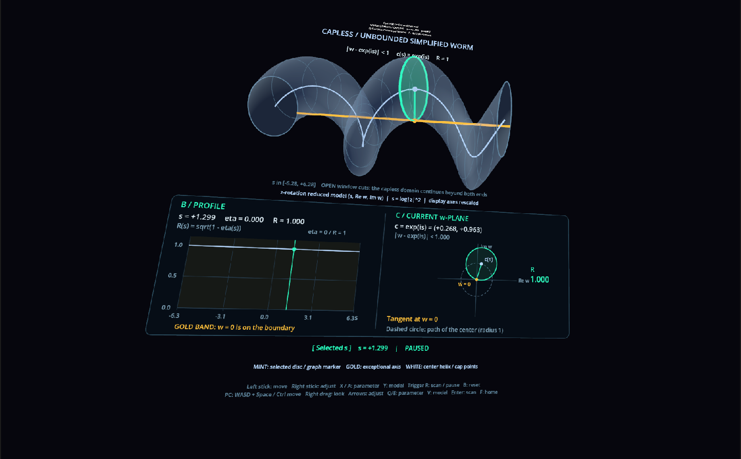
We join neighbouring sampled circles into a translucent boundary and highlight one filled disc. Every disc lies in a plane of constant \(s\); it is not a disc in the normal plane of the helix. On screen, \(s\) is the lengthwise direction, \(\operatorname{Im}w\) is height and \(\operatorname{Re}w\) is depth. Display scales and a fixed viewing tilt make the family easier to inspect.
隣り合う円周のサンプルをつないで半透明の境界を作り、選択した円板だけを面として強調します。各円板を置くのは \(s\) 一定の平面であり、螺旋の法平面ではありません。画面では \(s\) を長手方向、\(\operatorname{Im}w\) を高さ、\(\operatorname{Re}w\) を奥行きに割り当て、見やすい縮尺と傾きを付けています。
The display shows the domain and its boundary after symmetry reduction, not pseudoconvex neighbourhoods of its closure. We use the shape of the counterexample as a starting point for thinking about pseudoconvex neighbourhood bases for its closure.
表示しているのは領域と境界の対称性を縮約した姿で、閉包の擬凸近傍そのものではありません。ここでは、閉包の擬凸な基本近傍系について考える手掛かりとして、反例の形を観察します。
Starting with the unbounded version 非有界版から、境界の形を追う
The unbounded version considered in §2.3 of Xerakia’s preprint has no profile term. We call its display the capless model:
Xerakiaのプレプリントの§2.3で考察されている非有界版は、プロファイルの項を外した形です。今回の表示では、これをcaplessモデルと呼んでいます。
Now \(R(s)=1\) for every real \(s\). Since \(|0-e^{is}|=1\), the boundary of every disc passes through \(w=0\). These points form the gold axis \(\{(s,0,0):s\in\mathbb R\}\) in the reduced picture. As \(s\) changes, the centre moves around the origin, and the inward normal to the disc at the origin turns with it. This changing direction along the axis is the twist we are following.
この場合は、すべての実数 \(s\) で \(R(s)=1\) です。\(|0-e^{is}|=1\) なので、どの円板の境界も \(w=0\) を通ります。その点を並べたものが、金色の軸 \(\{(s,0,0):s\in\mathbb R\}\) です。\(s\) を変えると中心が原点の周りを移動し、原点から円板の内側へ向かう法線方向も変わります。この、軸に沿った方向の変化を「ねじれ」として追います。
Only a movable finite window is drawn: initially \(-2\pi\le s\le2\pi\). The two open ends are cuts made by the display window. They are not caps of this unbounded domain.
表示するのは動かせる有限の窓で、初期値は \(-2\pi\le s\le2\pi\) です。両端の開いた円周は、表示をそこで切った位置です。この非有界領域そのもののcapではありません。
Closing the ends 両端が閉じるまで
Making the discs shrink 円板を縮める函数
We fix a smooth, even, convex profile \(\eta\) satisfying the conditions above. It is zero on the central interval and flat to infinite order where it begins to increase. Its explicit construction is given in the implementation brief.
上の条件を満たす滑らかな偶凸函数 \(\eta\) を一つ選び、中央の零区間から増加し始める点で無限次に平坦になるようにつないでいます。具体的な函数の選び方は、実装依頼資料に記載しています。
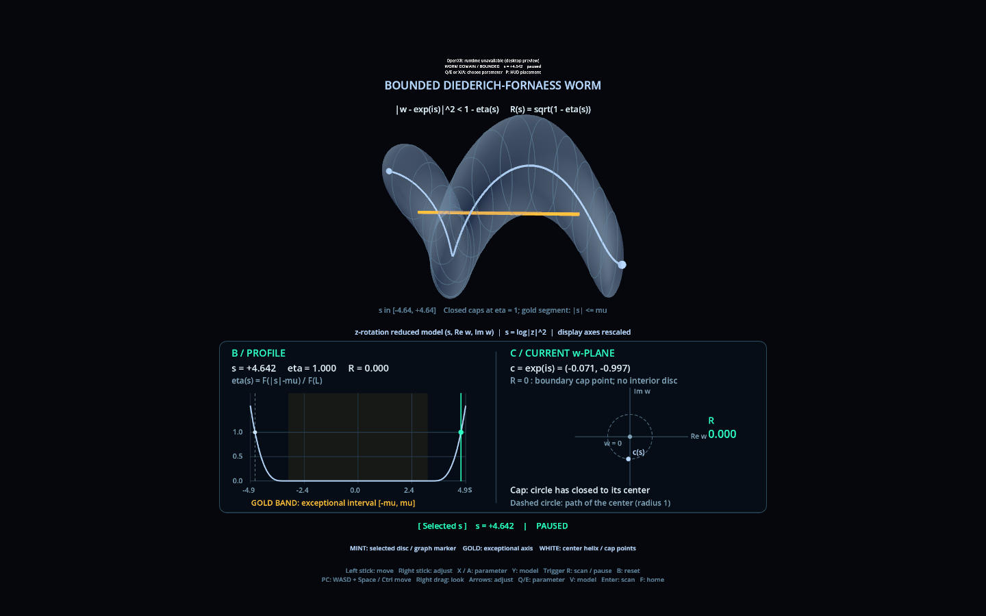
Outside the central interval, \(\eta\) increases and the disc radius \(R=\sqrt{1-\eta}\) decreases. Where \(\eta=1\), the open disc section is empty, while the boundary retains the point \(w=e^{is}\). This is the cap endpoint in the reduced view; beyond it there is no section.
中央区間の外では \(\eta\) が増え、円板の半径 \(R=\sqrt{1-\eta}\) が小さくなります。\(\eta=1\) となるところで開円板としての断面は空になり、境界には中心 \(w=e^{is}\) の一点が残ります。これが縮約した表示でのcapの端点で、その外には断面がありません。
Why the gold axis becomes a segment 金色の軸が、線分になる理由
In the central interval, the discs still have radius one and their boundaries pass through the origin. In the transition regions their radii are smaller than one, while their centres remain at distance one from the origin. The gold locus therefore stops at \(s=\pm\mu\), before the cap endpoints.
中央区間では、円板は半径1のままで、その境界が原点を通ります。一方、移行部分では半径が1より小さくなっても、中心から原点までの距離は1のままです。したがって金色の軌跡はcapの端点まで続かず、\(s=\pm\mu\) で終わります。
In the original domain, this is the exceptional annulus \(\mathcal A\); after quotienting by the \(z\)-rotation, it becomes the segment \(\mathcal A_{\mathrm{red}}\):
元の領域では、この部分は例外的な円環 \(\mathcal A\) です。\(z\) の回転対称性で割ると、線分 \(\mathcal A_{\mathrm{red}}\) として表示されます。
The boundary Levi form degenerates on this annulus; elsewhere the boundary is strongly pseudoconvex. The gold segment thus marks a feature of the complex geometry, not merely an axis chosen to organise the picture.
この円環では境界のLevi形式が退化し、それ以外の境界は強擬凸です。金色の線分は単なる表示上の補助軸ではなく、複素幾何の特徴を示す場所になっています。
Moving and comparing 動かして、見比べる
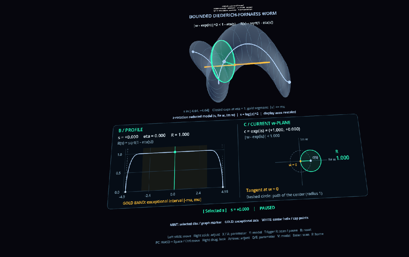
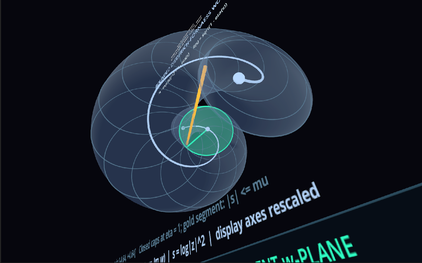
The mint disc in 3D, the mint graph marker, and the disc in the \(w\)-plane all use the same selected value \(s=s_0\). The pale helix marks the centres; the gold line or segment marks the exceptional locus. Lines, points and labels support the colour coding.
3Dのミント色の円板、グラフのミント色のマーカー、\(w\) 平面の円板は、同じ選択値 \(s=s_0\) を使います。白っぽい螺旋は中心の列、金色の直線・線分は例外的な軌跡です。色に加えて線幅、点、ラベルも手掛かりにしています。
As \(s\) varies in the capless model, the selected disc keeps touching the gold \(w=0\) axis, while its centre moves around the origin. We compare the 3D view with the \(w\)-plane to follow which side of the axis the domain occupies at each level.
caplessモデルで \(s\) を動かすと、選択円板は金色の \(w=0\) 軸に接したまま、中心が原点の周りを移動します。3D表示と \(w\) 平面を見比べることで、各高さで領域が軸のどちら側に広がるかを追います。
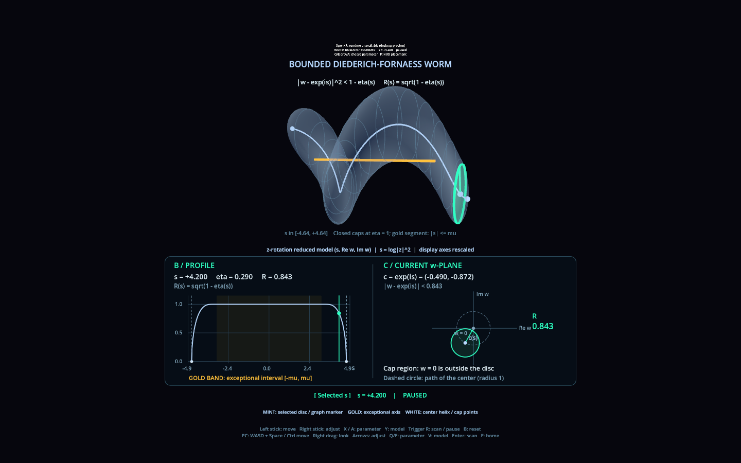
In the bounded model, the disc starts to shrink outside the central interval and no longer touches the axis. The gold segment therefore ends before the caps do. This distinguishes the weakly pseudoconvex annulus, seen as a segment, from the way the whole bounded domain closes at its ends.
boundedモデルでは、中央区間の外で円板が縮み始めると、円板は軸から離れます。そのため、金色の線分はcapより手前で終わります。線分として見えている弱擬凸な円環と、有界領域全体の両端の閉じ方とを分けて見られる点が、この比較の手掛かりです。
The graphs of \(\eta\) and \(R\) make the same change readable in the defining inequality. Near a cap, \(\eta\) approaches one as \(R\) approaches zero; the centre remains on the white helix.
\(\eta\) と \(R\) のグラフを並べると、同じ変化を定義不等式からも読めます。capに近づくにつれて \(\eta\) は1へ、\(R\) は0へ近づき、円板の中心は白い螺旋上に残ります。
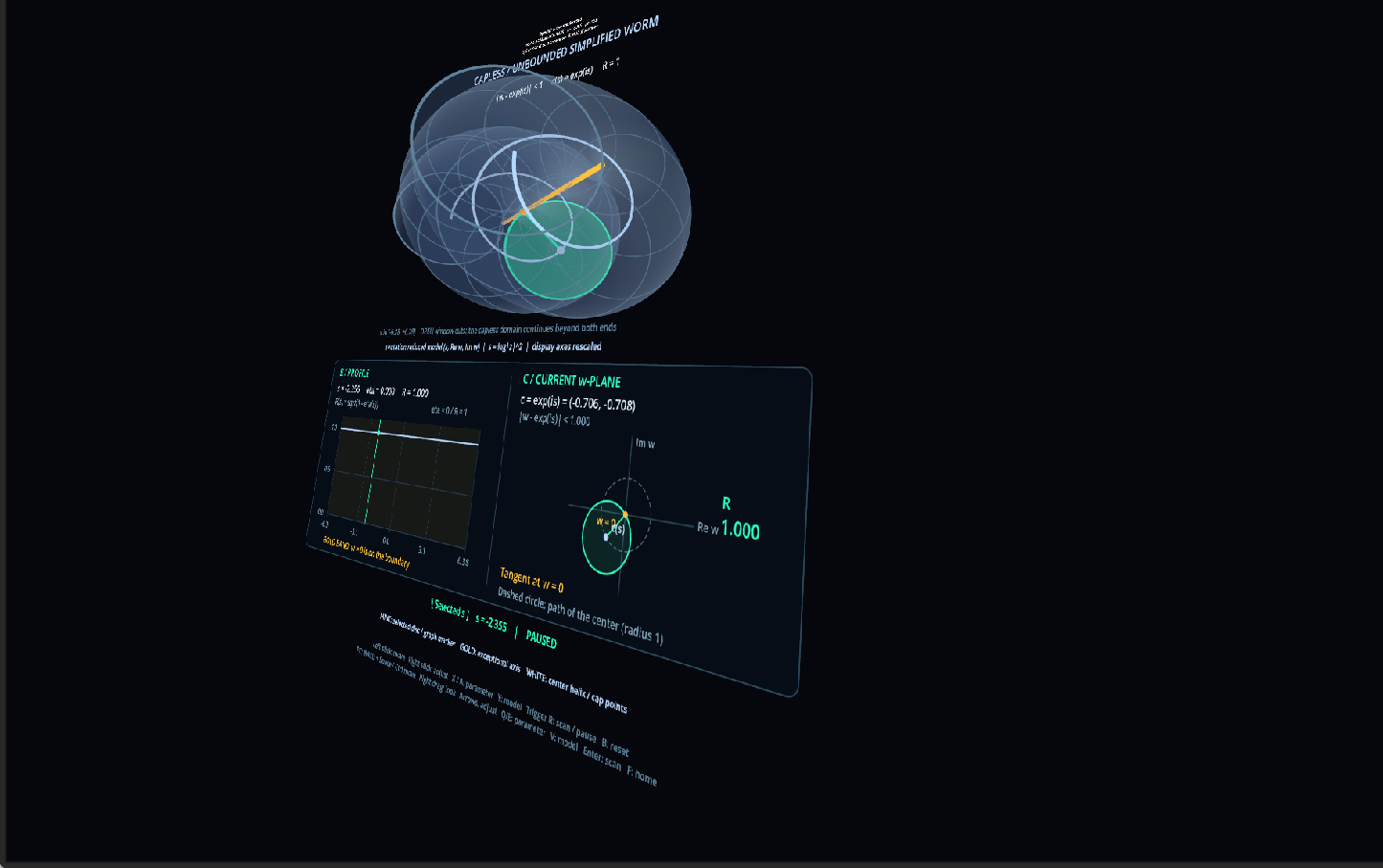
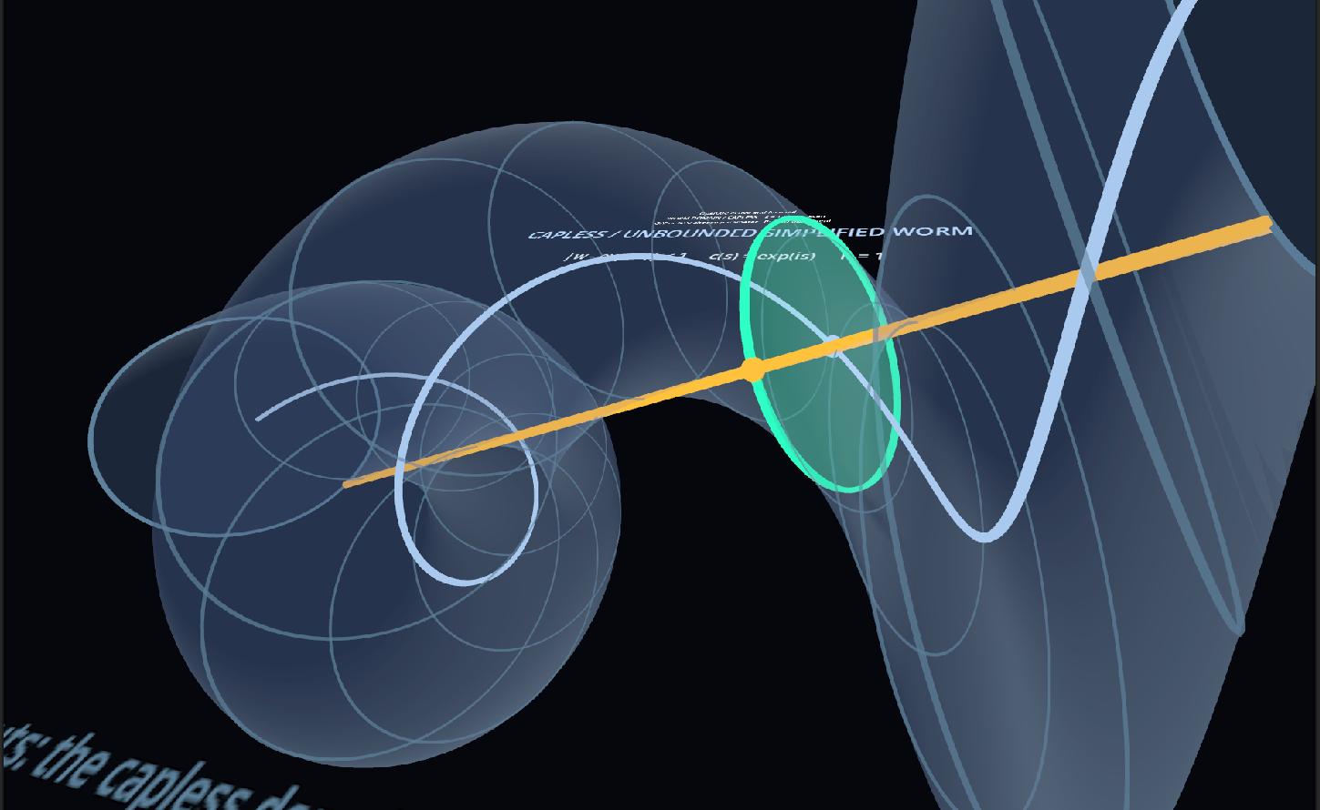
The following two desktop renders were saved separately during implementation checks. They complement the views above by showing a shrinking disc and the exact cap endpoint.
次の二枚は、実装確認の際に別途保存したPC描画です。上の画面を補うため、縮んだ円板と、ちょうどcapに達した位置を示します。
This web page records the application through still images; it does not run the VR application in the browser.
このWebページは、アプリの表示を静止画で紹介するページです。ブラウザー内でVRアプリを動かすものではありません。
Making it with Chapio-kun ちゃぴおくんと、どう作った?
We gave Chapio-kun a brief setting out the formulas and the intended views, and asked for an implementation making use of the general VR foundation. Codex implemented the disc family, the linked diagrams and the controls on that foundation.
数式と表示の狙いをまとめた依頼資料をちゃぴおくんに渡し、「汎用VR基本構成も活用しつつ」と実装をお願いしました。円板族と連動する図、操作部分は、Codexが既存の基本構成の上に実装しています。
The brief sets out the symmetry reduction, the capless and bounded models, and a candidate radius profile. Codex made these concrete through choices of boundary sampling, viewing tilt and panel layout, and reused the selection-colour conventions of the Levi-flat visualization.
依頼資料には、対称性による縮約、caplessとboundedの二つのモデル、半径を制御する函数の候補が記載されています。境界のサンプリング、見やすい傾き、連動パネルの配置、Levi平坦の表示と意味を揃えた色の利用などは、Codexが具体化した部分です。
After implementation, the project lead was able to view the capless model and then the bounded model. The images here record overviews, views along the axis and close observations.
実装後には、caplessモデルに続いてboundedモデルの表示も確認できました。掲載した画面は、全体像や軸に沿った向き、近づいた位置から見た記録です。
The brief and references 実装依頼資料と参考文献
The supplied September 2026 brief is preserved as TeX. A browser-readable HTML edition was made from it on 10 September 2026, retaining its original plans and mathematical text. The TeX is the source of the brief, not the application source code.
2026年9月の依頼資料を、受け取ったTeXのまま保存しています。ブラウザーで読めるHTML閲覧版は、2026年9月10日にその原本から作成し、当初の計画と数学の説明を残しました。TeXは依頼資料の文書ソースであり、アプリのソースコードではありません。
References参考文献
Klas Diederich and John Erik Fornæss, Pseudoconvex domains: an example with nontrivial Nebenhülle, Mathematische Annalen 225 (1977), 275–292. DOI: 10.1007/BF01425243.
The original source for the worm domain.
ワーム領域の原論文です。
-
F. Xerakia, Automorphisms of the worm domain, arXiv:2511.10614 (2025).
Our starting point is the unbounded version in §2.3. Definition 1 gives the bounded domain and the conditions on \(\eta\); §2.3 describes the exceptional annulus.
描画の出発点は§2.3の非有界版です。Definition 1では有界版の定義式と \(\eta\) の条件、§2.3では例外的な円環を参照しています。
See the setup guide, the note on implementation briefs, and our account of AI use.